
Do you want to learn the SUMIF formula in Excel in Hindi? If yes, then the wait is over now, because in this article I will give you information about SUMIF Formula in Excel in Hindi and english both with the practice file in detail. I’m going to give .
So if you also want to learn SUMIF Formula in Excel, then definitely read this article in full.
SUMIF formula in English
What is SUMIF formula in Excel?
Let’s first understand what is the SUMIF formula in Excel?
SUMIF formula is also called SUMIF function in Excel.
This is a very useful formula of Excel that we use to find the sum of a data based on a condition or criteria.
Syntax of SUMIF Formula in Excel
The syntax of sumif function in Excel is something like this:
=SUMIF(Range,Criteria,[Sum Range])
- Range: The range in which the criteria are to be applied.
- Criteria: Criteria or condition based on which you want to extract SUM.
- Sum range: The range from which you want to extract sum or total.
Note: If both criteria range and SUM range are the same, then sum range is not required in such a situation. Which you will learn in Example 3 below.
SUMIF Formula in Excel with 7 Examples
Below we have given 7 different types of examples of SUMIF Formula in Excel Hindi. After learning them, you can also download its practice file for practice.
Example 1: Text Criteria with SUMIF Formula in Excel
Now we will understand SUMIF through example. First of all, we will try to understand it with the simplest way text condition .
Suppose we have some kind of data as you see in the image below, in which region is written in column A and sales are given in other column B.
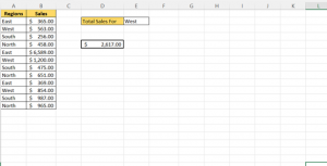
And you have been asked to find the total sales of West Region.
Our SUMIF formula will be something like this = SUMIF(A1:A13,” West”, B1:B13). And we will get the total sales of West Region 2617.
- Range: So first of all, we will select the range (A1:A13) in the SUMIF formula in which we want to put the condition.
- Criteria: And then write “West” in
- SUM Range: To find the total of West Region from sum range, select the range of sales (B1:B13).
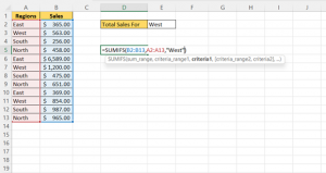
Keep one thing in mind that if we are using text in any formula in Excel, then we have to write it in Double Inverted Coma . Like I wrote “West” in this formula.
Example 3: Greater Than Criteria with SUMIF Formula in Excel in Hindi
Now we will try to understand sumif formula with greater than’s convention .
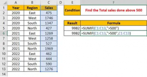
you have been asked to find the total of more than 500 sales.
So we will use the Greater Than sign >.
One thing to notice here is that the range in which the condition is to be applied and the range from which the sum is to be extracted are both the same.
And our SUMIF formula will be something like this =SUMIF(C1:C13,”>500″) or =SUMIF(C1:C13,”>500″,C1:C13). And we will get a total of 9942 sales of more than 500.
- Range: In our SUMIF formula, we will first select Range i.e. C1:C13
- Criteria: After that, we will write “>500” in the condition because we have to remove more than 500
- SUM Range: And whether we write SUM Range or not , it will not matter because both the range and sum range with condition are the same .
What is the SUMIFS Function in Excel in Hindi?
हम सभी जानते हैं कि SUMIF function हमें एक ही डेटा के भीतर संबंधित critirea के आधार पर दिए गए डेटा का योग देता है। हालांकि, एक्सेल में SUMIFS फ़ंक्शन कई criterias को लागू करने की अनुमति देता है।
Formula used for SUMIFS function in Excel in Hindi
“SUMIFs (sum_range, criteria_range1, Criteria 1, [criteria_range2, Criteria 2, criteria_range3, Criteria 3, … criteria_range_n, criteria_n] )”
Where:
Sum_range = जोड़ने के लिए cell range
Criteria_range1 = Range of cells जिस पर हम Ctriteria 1 लागू करना चाहते हैं
Criteria 1 = यह निर्धारित करने के लिए उपयोग किया जाता है कि कौन से cell जोड़ने हैं। criteria range 1 के आधार पर
Hindi translation.
Criteria_range2, Criteria 2, … = उनके संबंधित criterias के साथ additional cells
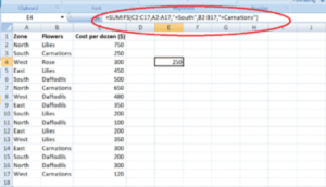
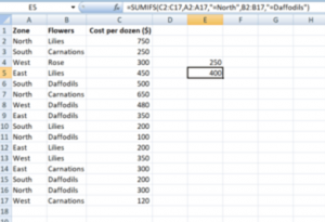
इसे समझने के लिए एक उदाहरण लेते हैं। मान लीजिए कि हम विभिन्न क्षेत्रों के लिए फूलों और प्रति दर्जन उनकी लागत के बारे में डेटा का उपयोग करते हैं। अगर मुझे south क्षेत्र के लिए carnation के लिए कुल लागत का पता लगाने की आवश्यकता है, तो मैं इसे निम्नलिखित तरीके से कर सकता हूं:
इसी तरह, अगर मैं northern क्षेत्र के लिए daffodils की कुल लागत का पता लगाना चाहता हूं, तो मैं उसी सूत्र का उपयोग कर सकता हूं।
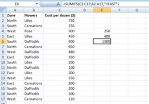
मान लीजिए कि मैं eastern क्षेत्र के लिए फूलों की कुल लागत का पता लगाना चाहता हूं, तो उपयोग किया जाने वाला सूत्र होगा:
SUMIFS फ़ंक्शन ‘=’, ‘>’, ‘<‘ जैसे तुलनात्मक ऑपरेटरों का उपयोग कर सकता है। यदि हम इन ऑपरेटरों का उपयोग करना चाहते हैं, तो हम उन्हें वास्तविक योग सीमा या किसी भी Criteria श्रेणियों पर लागू कर सकते हैं। इसके अलावा, हम उनका उपयोग करके तुलना ऑपरेटर बना सकते हैं:
- ‘< =’ (इससे कम या बराबर)
- ‘> =’ (इससे अधिक या बराबर)
- ‘<>’ (इससे कम या उससे अधिक/
आइए इसे विस्तार से समझने के लिए एक उदाहरण लेते हैं।
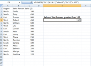
विभिन्न विक्रेताओं के प्रति क्षेत्र बिक्री के आंकड़ों का उपयोग करते हुए, मैं यह जानना चाहता हूं:
- 100 से अधिक उत्तर क्षेत्र की बिक्री
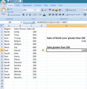
- 500 से अधिक की बिक्री
मैं निम्नानुसार उपर्युक्त ऑपरेटरों का उपयोग कर सकता हूं:
100 से अधिक north क्षेत्र की बिक्री
500 से अधिक की बिक्री
Use of wildcards
SUMIFS फ़ंक्शन का उपयोग करते समय Criteria के भीतर ‘*’ और ‘?’ जैसे wildcard वर्णों का उपयोग किया जा सकता है। इन वाइल्डकार्ड का उपयोग करने से हमें उन मैचों को खोजने में मदद मिलेगी जो एक समान हैं लेकिन सटीक मैच नहीं हैं।
Astric sign (*) को partial search का उपयोग करने की अनुमति देने के लिए criteria के बाद, पहले या आसपास के उपयोग किया जा सकता है।
उदाहरण के लिए, यदि मैं SUMIFS फ़ंक्शन में निम्न criteria लागू करता हूं:
- N * – इसका तात्पर्य range में सभी cells से है जो N से शुरू होते हैं
- * N – यह range में सभी cells का तात्पर्य है जो N के साथ समाप्त होता है
- * N * – cells जिनमें N होता है
Question mark (?) –
मान लीजिए कि मैं Criteria के रूप में NR लागू करता हूं। यहाँ “?” एक single character की जगह ले जाएगा। NR उत्तर, nar, आदि के साथ मेल खाएगा। हालाँकि, यह नाम को ध्यान में नहीं रखेगा।
क्या होगा यदि दी गई जानकारी में astric sign या question mark है?
इस मामले में, हम “टिल्ड (~)” का उपयोग कर सकते हैं। हमें उस परिदृश्य में प्रश्न चिह्न के सामने “~” टाइप करने की आवश्यकता है।